Running Stable Diffusion with Python - MachineLearningMastery.com

Stable Diffusion is a deep learning model that can generate pictures. In essence, it is a program in which you can provide input (such as a text prompt) and get back a tensor that represents an array of pixels, which, in turn, you can save as an image file. There’s no requirement that you must use a particular user interface. Before any user interface is available, you are supposed to run Stable Diffusion in code. In this tutorial, we will see how you can use the diffusers library from Hugging Face to run Stable Diffusion. After finishing this tutorial, you will learn - How to install the diffusers library and its dependencies - How to create a pipeline in diffusers - How to fine tune your image generation process Kick-start your project with my book Mastering Digital Art with Stable Diffusion. It provides self-study tutorials with working code. Let’s get started.  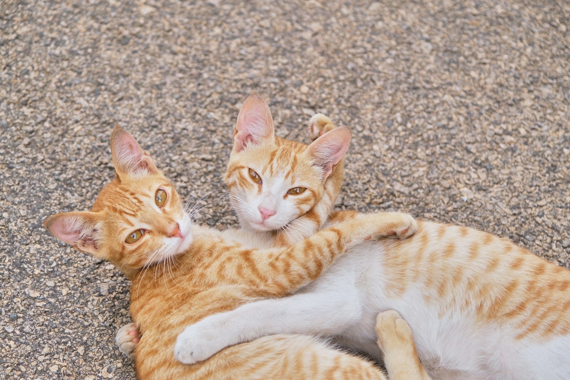Running Stable Diffusion in PythonPhoto by Himanshu Choudhary. Some rights reserved. ## Overview This tutorial is in three parts; they are - Introduction to the Diffusers Library - Customizing the Stable Diffusion Pipeline - Other Modules in the Diffusers Library ## Introduction to the Diffusers Library Stable Diffusion has taken the text-to-image generation world by storm. Its ability to produce high-quality, detailed images from textual descriptions makes it a powerful tool for artists, designers, and anyone with a creative spark. With the Stable Diffusion model file, you can rebuild the deep learning model using PyTorch, but you will need to write a lot of code to use it because there are many steps involved. The Hugging Face Diffusers library can harness Stable Diffusion’s potential and let you craft your own dreamlike creations. Before you use it, you should install the diffusers library in your Python environment: These Python packages have a lot of dependencies, including PyTorch. In this post, you will use the pipeline function in the diffuers library. It is called a pipeline because not a single deep learning model allows you to generate pictures from your input, but many smaller models work in tandem to achieve that. Let’s look at an example: | 12345678910111213141516 | from diffusers import StableDiffusionPipeline, DDPMSchedulerimport torchpipe = StableDiffusionPipeline.from_pretrained("CompVis/stable-diffusion-v1-4",variant="fp16", torch_dtype=torch.float16)pipe.to("cuda")prompt = "A cat took a fish and running in a market"scheduler = DDPMScheduler(beta_start=0.00085, beta_end=0.012,beta_schedule="scaled_linear")image = pipe(prompt,scheduler=scheduler,num_inference_steps=30,guidance_scale=7.5,).images[0]image.save("cat.png") | These are the few lines of code to generate a picture, and save it in PNG format to cat.png. 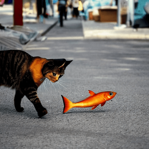This is an example of the generated picture:  A picture generated with Stable Diffusion pipeline. However, a lot of work is being done on the backend. You passed on a text prompt. This prompt has been converted into a numerical tensor using a pretrained embedding model. The tensor is then passed on to the Stable Diffusion model, downloaded from the Hugging Face repository “CompVis/stable-diffusion-v1-4” (the official Stable Diffusion v1.4 model). This model will be run with 30 steps and the DDPM scheduler. The output from the Stable Diffusion model will be a floating point tensor, which has to be converted into pixel values before you can save it. All these are accomplished by chaining the components with a pipeline into the object pipe. ## Customizing the Stable Diffusion Pipeline In the previous code, you download a pretrained model from the Hugging Face repository. Even for the same repository, different “variants” of the same model are available. Mostly, the default variant uses a 32-bit floating point, which is suitable for running on both CPU and GPU. The variant you used in the code above is fp16, which is to use 16-bit floating point. It is not always available and not always named as such. You should check the corresponding repository to learn more details. Because the variant used is for 16-bit floating point, you specified the torch_dtype to use torch.float16 as well. Note that most CPUs cannot work with 16-bit floating points (also known as half-precision floats), but it works for GPUs. Hence, you saw that the pipeline created was passed on to the GPU using the statement pipe.to("cuda"). You can try the following modification, which you should be able to observe a much slower generation because it is run on CPU: | 12345678910111213 | from diffusers import StableDiffusionPipeline, DDPMSchedulerpipe = StableDiffusionPipeline.from_pretrained("CompVis/stable-diffusion-v1-4")prompt = "A cat took a fish and running in a market"scheduler = DDPMScheduler(beta_start=0.00085, beta_end=0.012,beta_schedule="scaled_linear")image = pipe(prompt,scheduler=scheduler,num_inference_steps=30,guidance_scale=7.5,).images[0]image.save("cat.png") | However, suppose you have been using the Stable Diffusion Web UI and downloaded the third-party model for Stable Diffusion. In that case, you should be familiar with model files saved in SafeTensors format. This is in a different format than the above Hugging Face repository. Most notably, the repository would include a config.json file to describe how to use the model, but such information should be inferred from a SafeTensor model file instead. You can still use the model files you downloaded. For example, with the following code: | 123456789101112131415 | from diffusers import StableDiffusionPipeline, DDPMSchedulermodel = "./path/realisticVisionV60B1_v60B1VAE.safetensors"pipe = StableDiffusionPipeline.from_single_file(model)pipe.to("cuda")prompt = "A cat took a fish and running away from the market"scheduler = DDPMScheduler(beta_start=0.00085, beta_end=0.012,beta_schedule="scaled_linear")image = pipe(prompt,scheduler=scheduler,num_inference_steps=30,guidance_scale=7.5,).images[0]image.save("cat.png") | This code uses StableDiffusionPipeline.from_single_file() instead of StableDiffusionPipeline.from_pretrained(). The argument to this function is presumed to be the path to the model file. It will figure out that the file is in SafeTensors format. It is the neatness of the diffusers library that nothing else needs to be changed after you swapped how to create the pipeline. Note that each Pipeline assumes a certain architecture. For example, there is StableDiffusionXLPipeline from diffusers library solely for Stable Diffusion XL. You cannot use the model file with the wrong pipeline builder. You can see that the most important parameters of the Stable Diffusion image generation process are described in the pipe() function call when you triggered the process. For example, you can specify the scheduler, step size, and CFG scale. The scheduler indeed has another set of configuration parameters. You can choose among the many schedulers supported by the diffuers library, which you can find in the details in the diffusers API manual. For example, the following is to use a faster alternative, the Euler Scheduler, and keep everything else the same: | 123456789101112131415 | from diffusers import StableDiffusionPipeline, EulerDiscreteSchedulermodel = "./path/realisticVisionV60B1_v60B1VAE.safetensors"pipe = StableDiffusionPipeline.from_single_file(model)pipe.to("cuda")prompt = "A cat took a fish and running away from the market"scheduler = EulerDiscreteScheduler(beta_start=0.00085, beta_end=0.012,beta_schedule="scaled_linear")image = pipe(prompt,scheduler=scheduler,num_inference_steps=30,guidance_scale=7.5,).images[0]image.save("cat.png") | ## Other Modules in the Diffusers Library The StableDiffusionPipeline is not the only pipeline in the diffusers library. As mentioned above, you have StableDiffusionXLPipeline for the XL models, but there are much more. For example, if you are not just providing a text prompt but invoking the Stable Diffusion model with img2img, you have to use StableDiffusionImg2ImgPipeline. You can provide an image of the PIL object as an argument to the pipeline. You can check out the available pipelines from the diffusers documentation: - https://huggingface.co/docs/diffusers/main/en/api/pipelines/stable_diffusion/overview Even with the many different pipeline, you should find all of them work similarly. The workflow is highly similar to the example code above. You should find it easy to use without any need to understand the detailed mechanism behind the scene. ## Further Reading This section provides more resources on the topic if you want to go deeper. - diffusers API manual - Euler Scheduler API - DDPM Scheduler API In this post, you discovered how to use the diffusers library from Hugging Face. In particular, you learned: - How to create a pipeline to create an image from a prompt - How you can reuse your local model file instead of dynamically download from repository online - What other pipeline models are available from the diffusers library ## Get Started on Mastering Digital Art with Stable Diffusion! ### Learn how to make Stable Diffusion work for you ...by learning some key elements in the image generation process Discover how in my new Ebook: Mastering Digital Art with Stable Diffusion This book offers self-study tutorials complete with all the working code in Python, guiding you from a novice to an expert in image generation. It teaches you how to set up Stable Diffusion, fine-tune models, automate workflows, adjust key parameters, and much more...all to help you create stunning digital art. ### Kick-start your journey in digital art with hands-on exercises ### More On This Topic - Running and Passing Information to a Python Script  - Running a Neural Network Model in OpenCV  - A Technical Introduction to Stable Diffusion  - How to Create Images Using Stable Diffusion Web UI  - Prompting Techniques for Stable Diffusion  - Generate Realistic Faces in Stable Diffusion   Image by Author A loss function in machine learning is a mathematical formula that calculates the difference between the predicted output and the actual output of the model. The loss function is then used to slightly change the model weights and then check whether it has improved the model’s performance. The goal of machine learning algorithms is to minimize the loss function in order to make accurate predictions. In this blog, we will learn about the 5 most commonly used loss functions for classification and regression machine learning algorithms. ## 1. Binary Cross-Entropy Loss Binary cross-entropy loss, or Log loss, is a commonly used loss function for binary classification. It calculates the difference between the predicted probabilities and the actual labels. Binary cross-entropy loss is widely used for spam detection, sentiment analysis, or cancer detection, where the goal is to distinguish between two classes. The Binary Cross-Entropy loss function is defined as:  where y is the actual label (0 or 1), and ŷ is the predicted probability. In this formula, the loss function penalizes the model based on how far the predicted probability ŷ is from the actual target value y. ## 2. Hinge Loss Hinge loss is another loss function generally used for classification problems. It is often associated with Support Vector Machines (SVMs). Hinge loss calculates the difference between the predicted output and the actual label with a margin. The Hinge loss function is defined as:  where y is the true label (+1 or -1), and ŷ is the predicted output. The idea behind the Hinge loss is to penalize the model for misclassifications and being overly confident in its predictions. ## 3. Mean Square Error Mean Square Error (MSE) is the most common loss function used for regression problems. It calculates the average squared difference between predicted and actual values. The MSE loss function is defined as:  L(y, ŷ) = (1/n) * Σ(y_i - ŷ_i)^2 where: - n is the number of samples. - y is the true value of the i-th sample. 1 - ŷ is the predicted value of the i-th sample. i - Σ is the sum over all samples. The Mean square error is a measure of the quality of an algorithm. It is always non-negative, and values closer to zero are better. It is sensitive to outliers, meaning that a single very wrong prediction can significantly increase the loss. ## 4. Mean Absolute Error Mean Absolute Error (MAE) is another commonly used loss function for regression problems. It calculates the average absolute difference between predicted and actual values. The MAE loss function is defined as:  L(y, ŷ) = (1/n) * Σ|y_i - ŷ_i| where: - n is the number of samples. - y is the true value of the i-th sample. i - ŷ is the predicted value of the i-th sample. i - Σ is the sum over all samples. Similar to MSE, it is always non-negative, and values closer to zero are better. However, unlike the MSE, the MAE is less sensitive to outliers, meaning that a single very wrong prediction won’t significantly increase the loss. ## 5. Huber Loss Huber loss, also known as smooth mean absolute error, is a combination of Mean Square Error and Mean Absolute Error, making it a useful loss function for regression tasks, especially when dealing with noisy data. The Huber loss function is defined as:  where: - y is the actual value. - ŷ is the predicted value. - δ is a hyperparameter that controls the sensitivity to outliers. If the loss values are less than δ, use the MSE; if the loss values are greater than δ, use the MAE. It combines the best of both worlds from the two high-performance loss functions. MSE is excellent for detecting outliers, whereas MAE is great for ignoring them; Huber loss offers a balance between the two. ## Conclusion Just like how car headlights illuminate the road ahead, helping us navigate through the darkness and reach our destination safely, a loss function provides guidance to a machine learning algorithm, helping it navigate through the complex landscape of possible solutions and reach its optimal performance. This guidance helps in making adjustments to the model parameters to minimize error and improve accuracy, thereby steering the algorithm towards its optimal performance. In this blog, we have learned about 2 classification (Binary Cross-Entropy, Hinge) and 3 regression (Mean Square Error, Mean Absolute Error, Huber) loss functions. They are all popular functions for calculating the difference between predicted and actual values. ### More On This Topic - Loss and Loss Functions for Training Deep Learning Neural Networks  - How to Choose Loss Functions When Training Deep Learning Neural Networks  - How to Code the GAN Training Algorithm and Loss Functions  - A Gentle Introduction to Generative Adversarial Network Loss Functions  - A Gentle Introduction to XGBoost Loss Functions  - Loss Functions in TensorFlow